接上篇,一个ppo雏形,实现相对直观但缺乏工业级优化qaq根据openai这篇论文Proximal Policy Optimization Algorithms提出的内容进行了优化qwq
第一个版本里单环境采样效率低下,使用的是串行的gym.make(“CartPole-v1”),每次采样都在一个环境中逐步完成,单线程采样有训练效率瓶颈,速度慢的同时还容易导致样本相关性过高。PPO算法本质上依赖mini-batch SGD更新策略以减少方差,第一个版本直接使用整条trajectory进行 5 次完整passes更新,没有未进行随机打乱与分批处理。
第一个版本里我没有采用价值函数剪切 *value_loss = ((returns_tensor - values.squeeze()) * * 2).mean() *,直接使用均方误差作为价值函数回归目标,未采用PPO常用的 value clipping 技术,导致 critic 网络更新幅度过大进而影响 actor。
虽然第一个版本有早停机制,通过 KL 与 target_kl 比较,但是实现方式简单粗暴,逻辑是如果任意一个epoch中KL超阈值,整个episode的训练提前终止,非常容易造成梯度浪费。并且缺乏调度与动态调整机制,第一个版本代码中entropy_coef和其他超参数是固定值,不会随训练进度进行annealing。
综上,第二版本的优化思路是并行环境采样提升效率与样本多样性,用SyncVectorEnv创建8个并行环境来提升了采样效率和策略样本的多样性,通过collect_trajectory函数批量采样在较短时间内收集大量经验提升策略更新速度和减少样本间的时间相关性。
引入并行环境主要是为了缓解样本自相关性
在策略梯度类强化学习算法(如 PPO)中,智能体通过与环境交互获得状态-动作-奖励序列。若采用单线程串行环境采样,连续获得的样本往往在时间上强相关(即马尔可夫性下短时间内状态分布变化缓慢),这会导致采样分布退化、样本冗余、方差增大,从而影响策略估计的可靠性与训练收敛速度。为缓解这一问题,通常采用多环境并行采样(如 SyncVectorEnv 或 SubprocVectorEnv),即在多个独立环境中同时运行策略,每个环境状态的演化轨迹相对独立,从而增强经验多样性、降低样本间的时间依赖性。这一策略有效打破样本间的序列依赖结构,接近于 i.i.d.(独立同分布)假设,使得小批量 SGD 优化器能更有效地估计梯度,提高策略优化的鲁棒性与泛化能力。
env = SyncVectorEnv([make_env() for _ in range(8)])
这样每次更新都能在具有更多状态分布的经验下进行,符合论文中对于近似策略分布下最大化目标函数的假设。
在update_policy中我第二版引入了打乱+小批量训练minibatch SGD的机制,这是PPO的核心更新策略之一
idx = torch.randperm(len(obs_tensor))
for i in range(0, len(obs_tensor), minibatch_size):
    batch_idx = idx[i:i+minibatch_size]
第二个版本还引入Clipped Value Loss保证Critic的稳定训练,第一版是简单的MSE损失,第二版实现了论文的推荐机制——Clipped Value Function Loss来有效限制了critic更新的幅度避免critic对 eturns的过拟合。
value_pred_clipped = batch_val_old + (values.squeeze() - batch_val_old).clamp(-clip_eps, clip_eps)
value_loss1 = (values.squeeze() - batch_ret).pow(2)
value_loss2 = (value_pred_clipped - batch_ret).pow(2)
value_loss = 0.5 * torch.max(value_loss1, value_loss2).mean()
加入动态调整探索策略:Entropy 系数退火机制
entropy_coef = max(0.001, entropy_init * (1 - episode / num_episodes))
随着训练进展entropy_coef 逐渐减小从鼓励探索过渡到策略稳定阶段,有助于训练从 early exploration 平滑转向 final exploitation。
第二版代码使用了reward EMA平滑曲线与early best policy 保存机制,相比第一版只记录 reward 曲线,第二版还追踪表现最好的模型参数确保训练过程不仅关注 reward 上升趋势,也有后备策略可部署。
if smoothed_reward > best_reward:
    best_reward = smoothed_reward
    torch.save(net.state_dict(), "best_ppo_cartpole.pth")
在 compute_gae部分第二版采用了torch.zeros_like()向量化初始化并考虑了最后状态的 bootstrapped value,更贴近论文的时间差泛化优势估计理念。
时间差泛化优势估计(GAE)的本质理念是:通过结合多个时间尺度的 TD 残差,使用衰减加权平均(通过λ)得到更稳定的优势函数估计。它是一种在偏差-方差权衡中提供灵活控制的机制,增强了策略梯度方法的训练效果与稳定性,因此被 PPO 等先进算法广泛采用。
回到论文第三节如图。
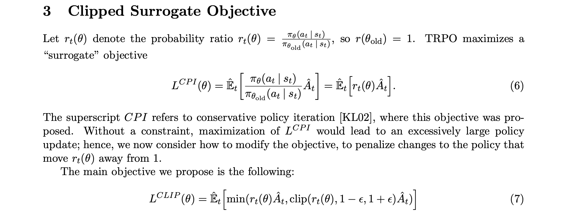
论文的提出源于对现有强化学习方法局限性,原文在引言中明确指出了三类主要方法的问题:”Q-learning (with function approximation) fails on many simple problems and is poorly understood, vanilla policy gradient methods have poor data efficiency and robustness; and trust region policy optimization (TRPO) is relatively complicated, and is not compatible with architectures that include noise (such as dropout) or parameter sharing“。特别是在策略梯度方法中原文强调了一个核心问题:”standard policy gradient methods perform one gradient update per data sample”
传统策略梯度方法使用的目标函数虽然在这个损失函数上使用相同轨迹进行多步优化很有吸引力,但“doing so is not well-justified, and empirically it often leads to destructively large policy updates”。
剪切机制的精妙之处我觉得是在于其对不同情况的差异化处理,论文通过图清晰地展示了剪切函数在正优势和负优势情况下的行为。当优势函数hat{A_t} > 0时,表示当前动作比平均水平好,此时如果概率比率r_t(theta) > 1 + epsilon,剪切机制会将其限制在1 + epsilon,防止对好动作的概率增加过度。相反当\hat{A_t} < 0时,表示动作比平均水平差,如果r_t(theta) < 1 - epsilon,剪切机制会将其限制在1 - epsilo防止对差动作的概率减少过度。
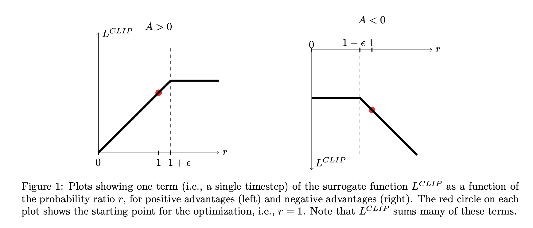
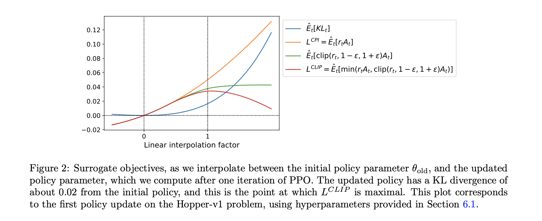
这种设计的核心哲学是保守主义”With this scheme, we only ignore the change in probability ratio when it would make the objective improve, and we include it when it makes the objective worse“,通过取最小值操作PPO确保了目标函数始终是未剪切目标的下界,形成了一个悲观估计。下图进一步验证了这一点L^{CLIP}确实是L^{CPI}的下界并且在KL散度约为0.02时达到最大值。
PPO算法的另一个关键创新是实现了在同一批数据上的多轮优化,第5节详细描述了算法实现:”Each iteration, each of N (parallel) actors collect T timesteps of data. Then we construct the surrogate loss on these NT timesteps of data, and optimize it with minibatch SGD (or usually for better performance, Adam), for K epochs“。
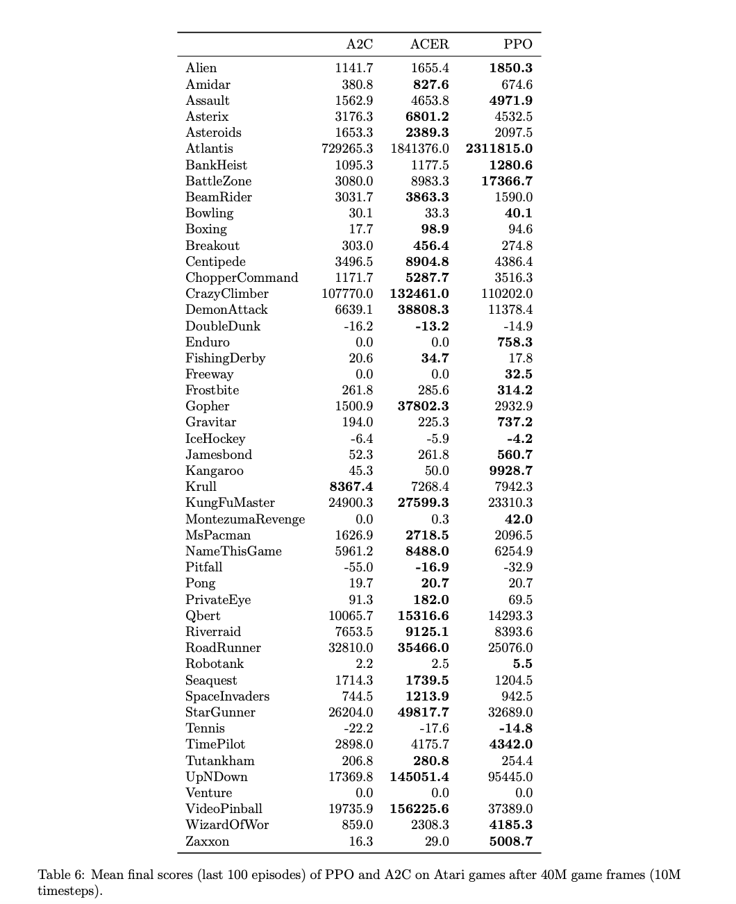
具体的实现流程:首先由N个并行actor各自收集T个时间步的数据,然后在这NT个样本上构建代理损失函数,使用小批量SGD进行K个epoch的优化,其中小批量大小M满足M leq NT,原文还强调了优化器的选择:”optimize it with minibatch SGD (or usually for better performance, Adam)“虽然理论上可以使用标准SGD但实践中Adam优化器通常能带来更好的性能。实验部分验证了这一优势在多个基准测试中都表现出了优于传统方法的样本复杂度。
优化后的colab代码
!pip install gymnasium[classic-control] torch matplotlib --quiet
import gymnasium as gym
import torch
import torch.nn as nn
import torch.optim as optim
import numpy as np
import matplotlib.pyplot as plt
from torch.distributions.categorical import Categorical
from tqdm.notebook import trange
from matplotlib import animation
from IPython.display import HTML, display
import os
from gymnasium.vector import SyncVectorEnv

class ActorCritic(nn.Module):
    def __init__(self, obs_dim, act_dim):
        super().__init__()
        self.shared = nn.Sequential(
            nn.Linear(obs_dim, 64), nn.ReLU(),
            nn.Linear(64, 64), nn.ReLU()
        )
        self.actor = nn.Linear(64, act_dim)
        self.critic = nn.Linear(64, 1)

    def forward(self, obs):
        x = self.shared(obs)
        return self.actor(x), self.critic(x)

def make_env():
    def thunk():
        return gym.make("CartPole-v1")
    return thunk

env = SyncVectorEnv([make_env() for _ in range(8)])
device = torch.device("cuda" if torch.cuda.is_available() else "cpu")

obs_dim = env.single_observation_space.shape[0]
act_dim = env.single_action_space.n
net = ActorCritic(obs_dim, act_dim).to(device)
optimizer = optim.Adam(net.parameters(), lr=1e-4)

def compute_gae(rewards, values, next_value, dones, gamma=0.99, lam=0.95):
    adv = torch.zeros_like(rewards).to(device)
    gae = 0
    for t in reversed(range(len(rewards))):
        delta = rewards[t] + gamma * next_value * (1 - dones[t]) - values[t]
        gae = delta + gamma * lam * (1 - dones[t]) * gae
        adv[t] = gae
        next_value = values[t]
    return adv

def collect_trajectory(env, net, buffer_limit):
    obs = env.reset()[0]
    done = np.zeros(env.num_envs)
    buffer = []
    steps = 0
    while steps < buffer_limit:
        obs_tensor = torch.tensor(obs, dtype=torch.float32).to(device)
        logits, value = net(obs_tensor)
        probs = Categorical(logits=logits)
        action = probs.sample()
        log_prob = probs.log_prob(action)

        next_obs, reward, terminated, truncated, _ = env.step(action.cpu().numpy())
        done_flag = np.logical_or(terminated, truncated)

        for i in range(env.num_envs):
            buffer.append((obs[i], action[i].item(), log_prob[i].item(), reward[i], value[i].item(), done_flag[i]))

        obs = next_obs
        done = done_flag
        steps += env.num_envs
    return buffer, obs

def update_policy(buffer, last_obs, net, optimizer, update_epochs, minibatch_size, clip_eps, entropy_coef, value_coef):
    obs_list, act_list, logp_list, rew_list, val_list, done_list = zip(*buffer)

    obs_tensor = torch.tensor(obs_list, dtype=torch.float32).to(device)
    act_tensor = torch.tensor(act_list).to(device)
    logp_tensor = torch.tensor(logp_list).to(device)
    val_tensor = torch.tensor(val_list, dtype=torch.float32).to(device)
    rew_tensor = torch.tensor(rew_list, dtype=torch.float32).to(device)
    done_tensor = torch.tensor(done_list, dtype=torch.float32).to(device)

    with torch.no_grad():
        last_obs_tensor = torch.tensor(last_obs, dtype=torch.float32).to(device)
        _, next_value = net(last_obs_tensor)
        next_value = next_value.mean(dim=0)

    adv_tensor = compute_gae(rew_tensor, val_tensor, next_value, done_tensor)
    returns_tensor = adv_tensor + val_tensor
    adv_tensor = (adv_tensor - adv_tensor.mean()) / (adv_tensor.std() + 1e-8)

    for _ in range(update_epochs):
        idx = torch.randperm(len(obs_tensor))
        for i in range(0, len(obs_tensor), minibatch_size):
            batch_idx = idx[i:i+minibatch_size]
            batch_obs = obs_tensor[batch_idx]
            batch_act = act_tensor[batch_idx]
            batch_adv = adv_tensor[batch_idx]
            batch_ret = returns_tensor[batch_idx]
            batch_logp_old = logp_tensor[batch_idx]
            batch_val_old = val_tensor[batch_idx]

            logits, values = net(batch_obs)
            probs = Categorical(logits=logits)
            new_logp = probs.log_prob(batch_act)
            entropy = probs.entropy().mean()

            ratio = (new_logp - batch_logp_old).exp()
            surr1 = ratio * batch_adv
            surr2 = torch.clamp(ratio, 1 - clip_eps, 1 + clip_eps) * batch_adv
            policy_loss = -torch.min(surr1, surr2).mean()

            value_pred_clipped = batch_val_old + (values.squeeze() - batch_val_old).clamp(-clip_eps, clip_eps)
            value_loss1 = (values.squeeze() - batch_ret).pow(2)
            value_loss2 = (value_pred_clipped - batch_ret).pow(2)
            value_loss = 0.5 * torch.max(value_loss1, value_loss2).mean()

            loss = policy_loss + value_coef * value_loss - entropy_coef * entropy

            optimizer.zero_grad()
            loss.backward()
            optimizer.step()

num_episodes = 2000
minibatch_size = 64
update_epochs = 4
clip_eps = 0.2
entropy_init = 0.02
value_coef = 0.5
reward_smoothing_alpha = 0.1
best_reward = -np.inf
rewards_history = []
smoothed_reward = 0
buffer_limit = 2048

def plot_metrics():
    plt.figure(figsize=(12, 6))
    plt.plot(rewards_history, label="Episode reward", alpha=0.4)
    ema_rewards = []
    ema = 0
    alpha = 0.1
    for r in rewards_history:
        ema = alpha * r + (1 - alpha) * ema
        ema_rewards.append(ema)
    plt.plot(ema_rewards, label="EMA Reward", color='orange')
    if len(rewards_history) >= 100:
        rolling_success = [np.mean(np.array(rewards_history[i:i+100]) >= 200) for i in range(len(rewards_history)-99)]
        plt.plot(range(99, len(rewards_history)), rolling_success, label="Success Rate (100ep window)", color='green')
    plt.xlabel("Episode")
    plt.ylabel("Reward / Success")
    plt.title("PPO Training Progress")
    plt.legend()
    plt.grid(True)
    plt.show()

for episode in trange(num_episodes):
    buffer, last_obs = collect_trajectory(env, net, buffer_limit)
    ep_reward = sum([transition[3] for transition in buffer]) / env.num_envs

    entropy_coef = max(0.001, entropy_init * (1 - episode / num_episodes))

    update_policy(buffer, last_obs, net, optimizer, update_epochs, minibatch_size, clip_eps, entropy_coef, value_coef)

    rewards_history.append(ep_reward)
    smoothed_reward = reward_smoothing_alpha * ep_reward + (1 - reward_smoothing_alpha) * smoothed_reward
    if smoothed_reward > best_reward:
        best_reward = smoothed_reward
        torch.save(net.state_dict(), "best_ppo_cartpole.pth")

plot_metrics()

def render_agent_as_gif(net, env, max_frames=500):
    frames = []
    obs, _ = env.reset()
    done = False

    for _ in range(max_frames):
        frame = env.render()
        frames.append(frame)

        obs_tensor = torch.tensor(obs, dtype=torch.float32).unsqueeze(0).to(device)
        with torch.no_grad():
            logits, _ = net(obs_tensor)
            probs = Categorical(logits=logits)
            action = probs.sample().item()

        obs, reward, terminated, truncated, _ = env.step(action)
        if terminated or truncated:
            break

    env.close()
    fig = plt.figure(figsize=(frames[0].shape[1] / 72, frames[0].shape[0] / 72), dpi=72)
    plt.axis("off")
    im = plt.imshow(frames[0])

    def update(frame):
        im.set_array(frame)
        return [im]

    ani = animation.FuncAnimation(fig, update, frames=frames, interval=30)
    html = ani.to_jshtml()
    plt.close()
    display(HTML(html))

render_env = gym.make("CartPole-v1", render_mode="rgb_array")
net.load_state_dict(torch.load("best_ppo_cartpole.pth"))
render_agent_as_gif(net, render_env)